1. Introduction

The skin effect is a well-known phenomenon in electrical engineering, particularly relevant to the performance of magnet wire in various applications. This effect, wherein alternating current (AC) tends to flow near the surface of a conductor at higher frequencies, leads to an increase in the effective resistance of the wire. Understanding and quantifying this effect is crucial for the design and optimization of electrical components such as transformers, inductors, and motors, where magnet wire is commonly used.
Wire gauge, which specifies the diameter of the wire, directly influences its electrical properties, including resistance and inductance. The relationship between wire gauge and resistance is fundamental to predicting the performance of electrical systems. However, the influence of frequency on this relationship, especially due to the skin effect, adds a layer of complexity that must be addressed for accurate modeling and design.
Through this investigation, the paper aims to provide a detailed understanding of the skin effect in magnet wire, offering valuable insights for engineers and researchers involved in the design and optimization of electrical systems.

2. Linear DC Resistance vs. Wire Gauge

The skin effect models the increase of resistance in a conductor as a function of frequency. There are many excellent papers and texts that cover the skin effect topic. Most of them focus on the physics behind the skin effect, however, many fall short providing practical guidance. This document will focus on practical tools instead of the physics.
The goal of this exercise is to provide a graphical representation of Magnet Wire effective resistance at various frequencies. In addition, providing the MathCad®™ worksheet will allow individuals to perform discrete evaluation at a particular frequency for a given wire size.
To that end, it is fortunate, and not well known, that wire gauge assignments are not random numbers assigned to randomly selected wire thicknesses.
The AWG assignments were made with precision and purpose.
It is no coincidence that 40 AWG copper magnet wire is and 10 AWG is 1

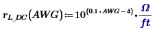
Equation 2–1: Linear DC resistance vs. Wire Gauge
The Values in the Graph below agrees with published wire charts.

Figure 2–1: Linear DC Resistance vs. Wire Gauge

2.1 Deriving Area and Circumference

Since the resistance (per foot) is known, the area and circumference can be derived if we introduce the DC resistivity of the coper alloy used in magnetic wire.

Dividing the resistivity by the resistance per foot (Equation 1) will yield the Area as a function of wire gauge



Equation 2–2: Wire Area as a function of Wire Gauge

Introducing the unit of circular mils (for area) becomes useful for comparison purposes since many published wire charts express wire area in circular mils. The term is just the square of the diameter in mils (0.001 inches).

Let’s test what we have so far at a few points...
   
These values agree with published data. Cooner Wire
From this the circumference can be calculated.
The circumference is related to Area by
Circumference can be written

Equation 2–3: Circumference as a function of Wire Gauge

2.2 Model 1 – Skin Effect Based on a Thin Wall Model

The surface resistance of the Magnet wire copper alloy as a function of frequency is presented below.

Equation 2–4: Surface Resistance in Ohms per Square

When the skin depth is much less than the wire radius, we can consider the conducting area as a thin walled pipe. We can mentally unroll the circumference into a flat plane. Dividing the AC resistance by the circumference yields the AC resistance per unit length.

Equation 2–5: Copper Wire Surface Resistance


Figure 2–2: Linear AC Resistance vs. Wire Gauge for Model 1

The graph compares the DC resistance to the AC resistance at various frequencies. It is interesting to note the different slopes. The DC resistance is governed by area ( ) while the AC resistance is governed by circumference ( ). The DC slope is 2 times the AC slope when plotted on a logarithmic scale.
The result is a sharpness to the graph when the effective depth is close to the radius of the wire.
This sharpness does not exist in nature.
To address this, a different model will be considered to smoothly transition from the AC curves to the DC curve.

2.3 Model 2 – Skin Effect Based on a Thick Wall Model

When the depth is about the same as the radius, the shape of the conducting area will be a very thick walled pipe. It would be more accurate to consider the cross sectional area for this geometry. The skin depth will be needed for this analysis. This will be the resistivity of the alloy divided by the AC resistance.

Equation 2–6: Effective Depth of Conduction


Figure 2–3: Linear AC Resistance

The resulting Area ( ) will be the area of the wire ( ) minus the area of the void ( ). The void is the area deeper than the effective skin depth.

Figure 2–4: Thick Wall Geometry







Equation 2–7: Effective Conducting Wire Area vs. Frequency

Equation 2–7 is now rewritten as a function

Dividing resistivity by the area will yield ohms/ft

Equation 2–8: Copper Wire Surface Resistance vs. Frequency


Figure 2–5: Linear AC Resistance vs. Wire Gauge for Model 2

3. Evaluation and Conclusion

3.1 Comparison of Models

Comparison of Model 1 (Thin wall) to Model 2 (Thick wall) yields similar results.


Both models give similar results when considering points far away from the intersection of the AC and DC lines. The benefit of Model 2 is that the AC curves meet the DC curve smoothly which better represents a natural process.

3.2 Comparison of Calculations to Measurements

Measurements were taken on different wire types at different frequencies. The error is less than 5% up to 500 kHz, and 12% up to 1 MHz.

Figure 3–1: Calculations vs. Measurements

3.3 Conclusion

Figure 2–5 provides a graphical estimation of AC resistance for Magnet wire.
It is relatively accurate for thin wall and thick wall models. Figure 2–2 is only accurate for thin wall models.